基于LightGBM实现保险反欺诈预测

项目以保险风控为背景，保险是重要的金融体系，对社会发展，民生保障起到重要作用。保险欺诈近些年层出不穷，在某些险种上保险欺诈的金额已经占到了理赔金额的20%甚至更多。对保险欺诈的识别成为保险行业中的关键应用场景。

一、项目背景

项目以保险风控为背景，保险是重要的金融体系，对社会发展，民生保障起到重要作用。保险欺诈近些年层出不穷，在某些险种上保险欺诈的金额已经占到了理赔金额的20%甚至更多。对保险欺诈的识别成为保险行业中的关键应用场景。

【任务】 数据集提供了之前客户索赔的车险数据，希望你能开发模型帮助公司预测哪些索赔是欺诈行为

【评价标准】 AUC, 即ROC曲线下面的面积 (Area under the Curve of ROC)

二、项目方案

1. 简述技术路线

流程：数据处理 →模型建模→训练→评估预测

在本次项目中，使用的数据集不存在缺失和重复，不用经过清洗和处理，使用sklearn完成模型建模和评估等操作，为完成预测任务采用了lightgbm进行模型训练。

2. Sklearn介绍 -机器学习最常用的一个库

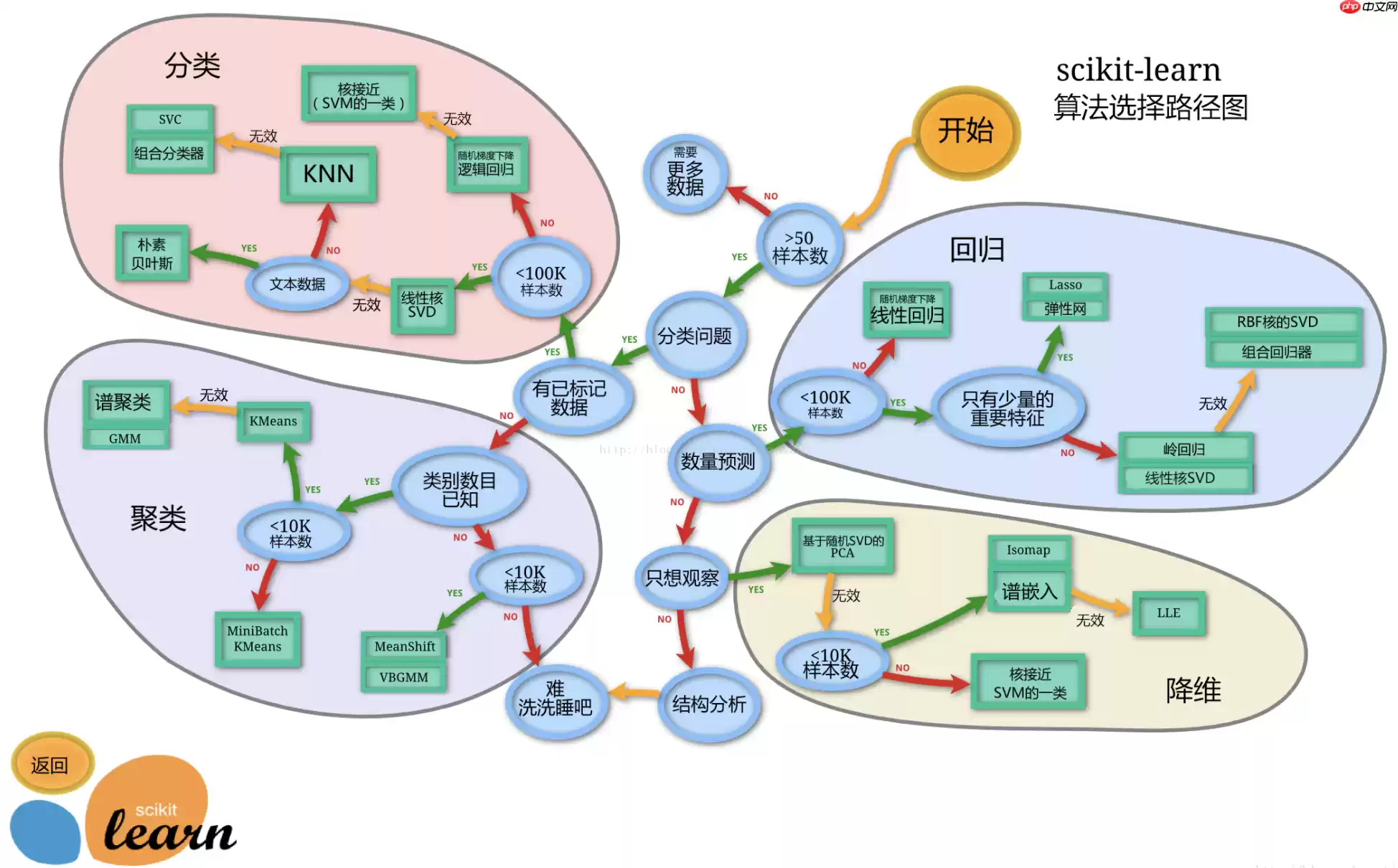
Sklearn 全称 Scikit-learn。它涵盖了分类、回归、聚类、降维、模型选择、数据预处理六大模块，降低机器学习实践门槛，将复杂的数学计算集成为简单的函数，并提供了众多公开数据集和学习案例。

正式中有详细的介绍：Sklearn最新文档

可以在AI Studio中进一步学习它:『行远见大』Python 进阶篇：Sklearn 库

下面是sklearn的算法选择路径，可供在模型选择中进行参考：

       

三、数据说明

挂载aistudio中的数据集：保险反欺诈预测

数据集内容：train.csv 训练集 test(1).csv 测试集 submission.csv 提交格式

通过载入数据集以及初步观察，对项目提供的数据集的表头进行理解和记录：

四、代码实现

共分为以下5个部分

1.数据集载入及初步观察

2.探索性数据分析

3.数据建模

4.模型评估

5.输出结果

下面将逐一进行介绍

1. 数据集载入及初步观察

In [1]

import pandas as pdimport numpy as npdf=pd.read_csv("保险反欺诈预测/train.csv")test=pd.read_csv("保险反欺诈预测/test (1).csv")df.head(10)

登录后复制        

   policy_id  age  customer_months policy_bind_date policy_state policy_csl  \0     122576   37              189       2013-08-21            C   500/1000   1     937713   44              234       1998-01-04            B    250/500   2     680237   33               23       1996-02-06            B   500/1000   3     513080   42              210       2008-11-14            A   500/1000   4     192875   29               81       2002-01-08            A    100/300   5     690246   47              305       1999-08-14            C    100/300   6     750108   48              308       2009-06-18            C    250/500   7     237180   30              103       2008-01-02            C   500/1000   8     300549   42               46       2010-11-12            A    100/300   9     532414   41              280       1998-11-10            B    250/500      policy_deductable  policy_annual_premium  umbrella_limit  insured_zip  ...  \0               1000                1465.71         5000000       455456  ...   1                500                 821.24               0       591805  ...   2               1000                1844.00               0       442490  ...   3                500                1867.29               0       439408  ...   4               1000                 816.25               0       640575  ...   5                500                1592.15               0       483650  ...   6               1000                1442.75         3000000       462503  ...   7               1000                1325.87               0       460080  ...   8               2000                 950.27               0       610944  ...   9               1000                1314.43         6000000       455585  ...     witnesses police_report_available total_claim_amount injury_claim  \0         3                       ?              54930         6029   1         1                     YES              50680         5376   2         1                      NO              47829         4460   3         2                     YES              68862        11043   4         1                     YES              59726         5617   5         2                      NO              57974        12975   6         0                      NO              53693         5731   7         2                     YES              63344        11427   8         3                       ?              74670        12864   9         3                     YES              55484         6128     property_claim  vehicle_claim  auto_make  auto_model auto_year fraud  0           5752          44452     Nissan      Maxima      2000     0  1          10156          37347      Honda       Civic      1996     0  2           9247          33644       Jeep    Wrangler      2002     0  3           5955          53548     Suburu      Legacy      2003     1  4          10301          41550       Ford        F150      2004     0  5           6619          39006       Saab          93      1996     1  6           5685          42042     Toyota  Highlander      2013     0  7           5429          43300     Suburu      Legacy      2012     0  8          20141          44657      Dodge         RAM      2004     1  9          12680          37788       Saab         92x      2007     0  [10 rows x 38 columns]

登录后复制                In [2]

#查看缺失值df.info()

登录后复制        

RangeIndex: 700 entries, 0 to 699Data columns (total 38 columns): #   Column                       Non-Null Count  Dtype  ---  ------                       --------------  -----   0   policy_id                    700 non-null    int64   1   age                          700 non-null    int64   2   customer_months              700 non-null    int64   3   policy_bind_date             700 non-null    object  4   policy_state                 700 non-null    object  5   policy_csl                   700 non-null    object  6   policy_deductable            700 non-null    int64   7   policy_annual_premium        700 non-null    float64 8   umbrella_limit               700 non-null    int64   9   insured_zip                  700 non-null    int64   10  insured_sex                  700 non-null    object  11  insured_education_level      700 non-null    object  12  insured_occupation           700 non-null    object  13  insured_hobbies              700 non-null    object  14  insured_relationship         700 non-null    object  15  capital-gains                700 non-null    int64   16  capital-loss                 700 non-null    int64   17  incident_date                700 non-null    object  18  incident_type                700 non-null    object  19  collision_type               700 non-null    object  20  incident_severity            700 non-null    object  21  authorities_contacted        700 non-null    object  22  incident_state               700 non-null    object  23  incident_city                700 non-null    object  24  incident_hour_of_the_day     700 non-null    int64   25  number_of_vehicles_involved  700 non-null    int64   26  property_damage              700 non-null    object  27  bodily_injuries              700 non-null    int64   28  witnesses                    700 non-null    int64   29  police_report_available      700 non-null    object  30  total_claim_amount           700 non-null    int64   31  injury_claim                 700 non-null    int64   32  property_claim               700 non-null    int64   33  vehicle_claim                700 non-null    int64   34  auto_make                    700 non-null    object  35  auto_model                   700 non-null    object  36  auto_year                    700 non-null    int64   37  fraud                        700 non-null    int64  dtypes: float64(1), int64(18), object(19)memory usage: 207.9+ KB

登录后复制        In [4]

# 绘制箱线图，查看异常值import matplotlib.pyplot as pltimport seaborn as sns# 分离数值变量与分类变量Nu_feature = list(df.select_dtypes(exclude=['object']).columns)  Ca_feature = list(df.select_dtypes(include=['object']).columns)# 绘制箱线图plt.figure(figsize=(30,30))   #  箱线图查看数值型变量异常值i=1for col in Nu_feature:    ax=plt.subplot(4,5,i)    ax=sns.boxplot(data=df[col])    ax.set_xlabel(col)    ax.set_ylabel('Frequency')    i+=1plt.show()# 结合原始数据及经验，真正的异常值只有umbrella_limit这一个变量，有一个-1000000的异常值，但测试集没有，可以忽略不管

登录后复制        

登录后复制                

2. 探索性数据分析

查看训练集与测试集数值变量分布

查看分类变量分布

查看数据相关性

查看训练集与测试集数值变量分布

In [5]

#查看训练集与测试集数值变量分布import warningswarnings.filterwarnings("ignore")plt.figure(figsize=(20,15))i=1Nu_feature.remove('fraud')for col in Nu_feature:    ax=plt.subplot(4,5,i)    ax=sns.kdeplot(df[col],color='red')    ax=sns.kdeplot(test[col],color='cyan')    ax.set_xlabel(col)    ax.set_ylabel('Frequency')    ax=ax.legend(['train','test'])    i+=1plt.show()

登录后复制        

登录后复制                

查看分类变量分布

In [6]

# 查看分类变量分布col1=Ca_featureplt.figure(figsize=(40,40))j=1for col in col1:    ax=plt.subplot(8,5,j)    ax=plt.scatter(x=range(len(df)),y=df[col],color='red')    plt.title(col)    j+=1k=11for col in col1:    ax=plt.subplot(5,8,k)    ax=plt.scatter(x=range(len(test)),y=test[col],color='cyan')    plt.title(col)    k+=1plt.subplots_adjust(wspace=0.4,hspace=0.3)  plt.show()

登录后复制        

登录后复制                

查看数据相关性

In [7]

from sklearn.preprocessing import LabelEncoderlb = LabelEncoder()                               cols = Ca_featurefor m in cols:    df[m] = lb.fit_transform(df[m])    test[m] = lb.fit_transform(test[m])correlation_matrix=df.corr()plt.figure(figsize=(12,10))sns.heatmap(correlation_matrix,vmax=0.9,linewidths=0.05,cmap="RdGy")# 几个相关性比较高的特征在模型的特征输出部分也占据比较重要的位置

登录后复制        

登录后复制                

登录后复制                

3. 数据建模

切割训练集和测试集

这里使用留出法划分数据集，将数据集分为自变量和因变量。

按比例切割训练集和测试集(一般测试集的比例有30%、25%、20%、15%和10%)，使用分层抽样，设置随机种子以便结果能复现

x_train,x_test,y_train,y_test = train_test_split( X, Y,test_size=0.3,random_state=1)

登录后复制        模型创建

创建基于树的分类模型（lightgbm）

这些模型进行训练，分别的到训练集和测试集的得分

In [8]

from lightgbm.sklearn import LGBMClassifierfrom sklearn.model_selection import train_test_splitfrom sklearn.model_selection import KFoldfrom sklearn.metrics import accuracy_score, auc, roc_auc_scoreX=df.drop(columns=['policy_id','fraud'])Y=df['fraud']test=test.drop(columns='policy_id')# 划分训练及测试集x_train,x_test,y_train,y_test = train_test_split( X, Y,test_size=0.3,random_state=1)

登录后复制    In [19]

# 建立模型gbm = LGBMClassifier(n_estimators=600,learning_rate=0.01,boosting_type= 'gbdt',       objective = 'binary',    max_depth = -1,      random_state=2024,               metric='auc')

登录后复制    

4. 模型评估

交叉验证介绍

交叉验证（cross-validation）是一种评估泛化性能的统计学方法，它比单次划分训练集和测试集的方法更加稳定、全面。在交叉验证中，数据被多次划分，并且需要训练多个模型。最常用的交叉验证是 k 折交叉验证（k-fold cross-validation），其中 k 是由用户指定的数字，通常取 5 或 10。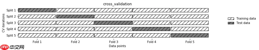            In [10]

# 交叉验证result1 = []mean_score1 = 0n_folds=5kf = KFold(n_splits=n_folds ,shuffle=True,random_state=2024)for train_index, test_index in kf.split(X):    x_train = X.iloc[train_index]    y_train = Y.iloc[train_index]    x_test = X.iloc[test_index]    y_test = Y.iloc[test_index]    gbm.fit(x_train,y_train)    y_pred1=gbm.predict_proba((x_test),num_iteration=gbm.best_iteration_)[:,1]    print('验证集AUC:{}'.format(roc_auc_score(y_test,y_pred1)))    mean_score1 += roc_auc_score(y_test,y_pred1)/ n_folds    y_pred_final1 = gbm.predict_proba((test),num_iteration=gbm.best_iteration_)[:,1]    y_pred_test1=y_pred_final1    result1.append(y_pred_test1)

登录后复制        

验证集AUC:0.8211382113821137验证集AUC:0.8088235294117647验证集AUC:0.8413402315841341验证集AUC:0.8452820891845282验证集AUC:0.8099856321839081

登录后复制        In [20]

# 模型评估print('mean 验证集auc:{}'.format(mean_score1))cat_pre1=sum(result1)/n_folds

登录后复制        

mean 验证集auc:0.8253139387492898

登录后复制        

5. 输出结果

将预测结果按照指定格式输出到submission-Copy2.csv文件中

In [21]

ret1=pd.DataFrame(cat_pre1,columns=['fraud'])ret1['fraud']=np.where(ret1['fraud']>0.5,'yes','no').astype('str')result = pd.DataFrame()result['policy_id'] = df['policy_id']result['fraud'] = ret1['fraud']result.to_csv('/home/aistudio/submission.csv',index=False)

登录后复制    

五、效果展示

最后得到验证集accuracy达到0.8253139387492898