大语言模型已经席卷全球,从 GPT 到 LLaMA,参数量动辄数十亿甚至万亿。但在实际部署中,显存、延迟、成本、能耗,哪个都不是省油的灯。怎么让这些庞然大物在消费级显卡上跑起来?答案就是模型量化——用更低精度的数值表示,换取存储、速度和功耗的全面提升。下面我们来系统梳理量化的来龙去脉,从最基础的线性量化,到 GPTQ、AWQ 这类大模型专用方法,再到 GGUF 这类本地推理格式,最后给出选型指南。
一、引言:为什么需要模型量化?
1.1 大模型部署的痛点
随着 GPT、LLaMA、DeepSeek 等大语言模型的兴起,模型规模呈指数级增长:
模型 | 参数量 | FP16 显存占用 | 推理成本 |
|---|---|---|---|
GPT-2 | 1.5B | 3 GB | 低 |
LLaMA-2-7B | 7B | 14 GB | 中 |
LLaMA-2-70B | 70B | 140 GB | 高 |
GPT-4 | ~1.8T | ~3.6 TB | 极高 |
核心挑战:
• 显存瓶颈: 消费级 GPU(如 RTX 4090 24GB)无法加载 70B 模型• 推理延迟: 大模型生成速度慢,用户体验差
• 部署成本: 云端推理费用高昂,边缘部署困难
• 能耗问题: 大模型推理功耗高,不利于移动设备
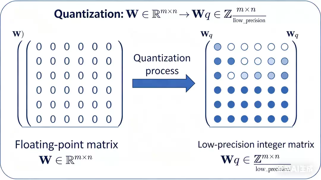
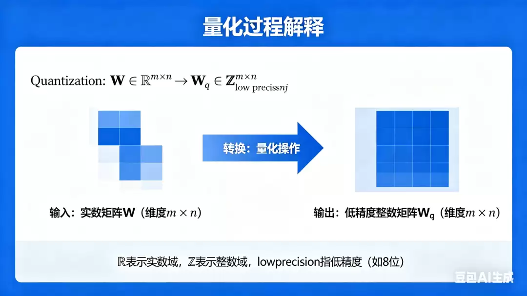
1.2 模型量化的核心思想
模型量化(Model Quantization) 是将模型参数从高精度(如 FP32/FP16)转换为低精度(如 INT8/INT4)表示的技术:
量化收益:
• 存储减少: INT8 比 FP16 减少 50%,INT4 减少 75%• 速度提升: 低精度运算更快,支持专用硬件加速
• 功耗降低: 内存访问和计算能耗显著下降
精度 | 位数 | 相对存储 | 典型加速比 |
|---|---|---|---|
FP32 | 32 | 100% | 1x |
FP16 | 16 | 50% | 1.5-2x |
BF16 | 16 | 50% | 1.5-2x |
INT8 | 8 | 25% | 2-4x |
INT4 | 4 | 12.5% | 4-8x |
INT2 | 2 | 6.25% | 8-16x |
1.3 量化的挑战
量化并非免费午餐,主要挑战包括:
- 精度损失: 低精度表示导致模型能力下降
- 动态范围: 激活值分布范围广,难以均匀量化
- 异常值: 大模型中存在离群值(outliers),影响量化效果
- 任务敏感: 不同任务对量化敏感度不同
二、量化基础:线性量化与对称/非对称量化
2.1 线性量化公式
线性量化是最基础的量化方法,将浮点数映射到整数:
其中:
• (scale): 缩放因子• (zero point): 零点偏移
• : 四舍五入取整
反量化:
2.2 对称量化 vs 非对称量化
对称量化(Symmetric Quantization)
假设权重分布关于零点对称,零点偏移 :
优点: 计算简单,无需处理零点偏移
缺点: 无法很好地处理非对称分布
非对称量化(Asymmetric Quantization)
考虑权重分布的不对称性:
优点: 适应任意分布,精度更高
缺点: 计算稍复杂,需要处理零点
2.3 代码实现:基础量化器
代码语言:ja vascript复制import torch
import numpy as np
class LinearQuantizer:
"""线性量化器(支持对称/非对称)"""
def __init__(self, bits=8, symmetric=True):
self.bits = bits
self.symmetric = symmetric
if symmetric:
self.qmin = -(2 ** (bits - 1))
self.qmax = 2 ** (bits - 1) - 1
else:
self.qmin = 0
self.qmax = 2 ** bits - 1
def compute_scale_zero_point(self, tensor):
"""计算 scale 和 zero_point"""
if self.symmetric:
abs_max = torch.max(torch.abs(tensor))
scale = abs_max / self.qmax
zero_point = 0
else:
min_val = torch.min(tensor)
max_val = torch.max(tensor)
scale = (max_val - min_val) / (self.qmax - self.qmin)
zero_point = self.qmin - torch.round(min_val / scale)
return scale, zero_point
def quantize(self, tensor):
"""量化张量"""
scale, zero_point = self.compute_scale_zero_point(tensor)
quantized = torch.round(tensor / scale + zero_point)
quantized = torch.clamp(quantized, self.qmin, self.qmax)
return quantized.to(torch.int8 if self.bits == 8 else torch.int32), scale, zero_point
def dequantize(self, quantized, scale, zero_point):
"""反量化"""
return scale * (quantized.float() - zero_point)
def quantize_dequantize(self, tensor):
"""量化后立即反量化(模拟量化效果)"""
quantized, scale, zero_point = self.quantize(tensor)
return self.dequantize(quantized, scale, zero_point)
# 使用示例
print("=" * 60)
print("基础线性量化演示")
print("=" * 60)
weight = torch.randn(10, 10) * 2
quantizer_sym = LinearQuantizer(bits=8, symmetric=True)
quantized_sym, scale_sym, zp_sym = quantizer_sym.quantize(weight)
weight_dequant_sym = quantizer_sym.dequantize(quantized_sym, scale_sym, zp_sym)
quantizer_asym = LinearQuantizer(bits=8, symmetric=False)
quantized_asym, scale_asym, zp_asym = quantizer_asym.quantize(weight)
weight_dequant_asym = quantizer_asym.dequantize(quantized_asym, scale_asym, zp_asym)
error_sym = torch.mean(torch.abs(weight - weight_dequant_sym)).item()
error_asym = torch.mean(torch.abs(weight - weight_dequant_asym)).item()
print(f"原始权重范围: [{weight.min():.4f}, {weight.max():.4f}]")
print(f"对称量化 - 平均绝对误差: {error_sym:.6f}")
print(f"非对称量化 - 平均绝对误差: {error_asym:.6f}")
print(f"存储节省: {(32 - 8) / 32 * 100:.1f}%")
三、训练后量化(PTQ):零成本压缩
3.1 PTQ 概述
训练后量化(Post-Training Quantization, PTQ) 是最简单的量化方法:
• 无需重新训练: 直接对预训练模型进行量化• 快速部署: 几分钟内完成模型转换
• 适用场景: 快速验证、资源受限环境
PTQ 流程:
代码语言:ja vascript复制预训练模型 (FP32/FP16)
↓
收集校准数据(少量样本)
↓
计算每层 scale 和 zero_point
↓
量化权重和激活
↓
部署量化模型 (INT8/INT4)
3.2 动态范围量化
动态范围量化(Dynamic Range Quantization) 在推理时动态计算激活的量化参数:
代码语言:ja vascript复制import torch
import torch.quantization
model = torch.nn.Sequential(
torch.nn.Linear(784, 256),
torch.nn.ReLU(),
torch.nn.Linear(256, 10)
)
model_quantized = torch.quantization.quantize_dynamic(
model,
{torch.nn.Linear},
dtype=torch.qint8
)
print(f"原始模型参数数量: {sum(p.numel() for p in model.parameters())}")
print(f"量化后模型类型: {type(model_quantized)}")
特点:
• 权重静态量化,激活动态量化• 实现简单,但推理时需要计算统计量
• 适合对延迟不敏感的场景
3.3 静态量化
静态量化(Static Quantization) 使用校准数据集预先计算激活的量化参数:
代码语言:ja vascript复制class StaticQuantizationExample:
"""静态量化完整示例"""
def __init__(self, model):
self.model = model
def prepare_for_quantization(self):
self.model.qconfig = torch.quantization.get_default_qconfig('fbgemm')
torch.quantization.prepare(self.model, inplace=True)
return self.model
def calibrate(self, calibration_data):
self.model.eval()
with torch.no_grad():
for batch in calibration_data:
self.model(batch)
def convert_to_quantized(self):
torch.quantization.convert(self.model, inplace=True)
return self.model
校准数据选择:
• 通常使用 100-1000 个代表性样本• 应覆盖模型可能遇到的各种输入分布
• 过多校准数据收益递减
3.4 PTQ 的局限性
问题 | 原因 | 影响 |
|---|---|---|
精度损失大 | 未考虑量化对训练目标的影响 | 任务性能下降 |
异常值敏感 | 离群值主导动态范围 | 大部分数值精度降低 |
层间误差累积 | 每层独立量化,误差传播 | 深层网络更严重 |
四、量化感知训练(QAT):精度与效率的平衡
4.1 QAT 核心思想
量化感知训练(Quantization-Aware Training, QAT) 在训练过程中模拟量化效果,让模型学习适应量化误差:
代码语言:ja vascript复制标准训练: 前向(FP32) → 反向 → 更新
QAT训练:
前向(FP32→模拟量化→FP32) → 反向 → 更新
关键洞察: 在训练时引入量化噪声,模型可以学习更鲁棒的权重表示。
4.2 伪量化(Fake Quantization)
QAT 使用伪量化模拟低精度运算:
特点:
• 前向传播:模拟量化效果• 反向传播:使用 Straight-Through Estimator (STE) 传递梯度
4.3 STE(直通估计器)
量化函数的梯度几乎处处为0,无法直接反向传播。STE 的解决方案是:
即忽略量化函数,直接传递梯度。
代码语言:ja vascript复制class FakeQuantize(torch.nn.Module):
"""伪量化模块(支持 STE)"""
def __init__(self, bits=8, symmetric=True):
super().__init__()
self.bits = bits
self.symmetric = symmetric
if symmetric:
self.qmin = -(2 ** (bits - 1))
self.qmax = 2 ** (bits - 1) - 1
else:
self.qmin = 0
self.qmax = 2 ** bits - 1
self.scale = torch.nn.Parameter(torch.ones(1))
self.zero_point = torch.nn.Parameter(torch.zeros(1))
def forward(self, x):
if self.training:
return FakeQuantizeSTE.apply(x, self.scale, self.zero_point, self.qmin, self.qmax)
else:
return self._quantize(x)
def _quantize(self, x):
x_quant = torch.round(x / self.scale + self.zero_point)
x_quant = torch.clamp(x_quant, self.qmin, self.qmax)
return self.scale * (x_quant - self.zero_point)
class FakeQuantizeSTE(torch.autograd.Function):
@staticmethod
def forward(ctx, x, scale, zero_point, qmin, qmax):
x_quant = torch.round(x / scale + zero_point)
x_quant = torch.clamp(x_quant, qmin, qmax)
return scale * (x_quant - zero_point)
@staticmethod
def backward(ctx, grad_output):
return grad_output, None, None, None, None
4.4 QAT 完整训练流程
代码语言:ja vascript复制class QATModel(torch.nn.Module):
"""支持 QAT 的模型"""
def __init__(self, input_dim, hidden_dim, output_dim):
super().__init__()
self.fc1 = torch.nn.Linear(input_dim, hidden_dim)
self.fake_quant1 = FakeQuantize(bits=8)
self.relu = torch.nn.ReLU()
self.fc2 = torch.nn.Linear(hidden_dim, output_dim)
self.fake_quant2 = FakeQuantize(bits=8)
def forward(self, x):
x = self.fc1(x)
x = self.fake_quant1(x)
x = self.relu(x)
x = self.fc2(x)
x = self.fake_quant2(x)
return x
def train_qat(model, train_loader, num_epochs=10):
optimizer = torch.optim.Adam(model.parameters(), lr=1e-3)
criterion = torch.nn.CrossEntropyLoss()
print("阶段1:正常训练...")
print("阶段2:启用量化感知训练...")
for epoch in range(num_epochs):
model.train()
total_loss = 0
for batch_idx, (data, target) in enumerate(train_loader):
optimizer.zero_grad()
output = model(data)
loss = criterion(output, target)
loss.backward()
optimizer.step()
total_loss += loss.item()
print(f"Epoch {epoch+1}/{num_epochs}, Loss: {total_loss/len(train_loader):.4f}")
print("阶段4:转换为量化模型...")
quantized_model = convert_to_real_quantization(model)
return quantized_model
def convert_to_real_quantization(model):
model.eval()
return model
4.5 PTQ vs QAT 对比
特性 | PTQ | QAT |
|---|---|---|
训练成本 | 无 | 需要微调 |
精度损失 | 较大(2-5%) | 较小(0.5-2%) |
实现复杂度 | 简单 | 较复杂 |
适用场景 | 快速部署、资源充足 | 精度敏感、生产环境 |
典型工具 | TensorRT, ONNX Runtime | PyTorch QAT, TensorFlow Lite |
五、GPTQ:大模型量化的突破
5.1 背景:大模型量化的挑战
LLM(大语言模型)的量化面临独特挑战:
- 参数量巨大: 70B 模型即使 INT4 也需要 35GB 存储
- 异常值问题: 激活中存在大量离群值(outliers)
- 层间依赖: Transformer 层间有残差连接,误差会传播
传统 PTQ/QAT 在大模型上效果不佳,需要新的量化范式。
5.2 GPTQ 核心思想
GPTQ(Generative Pre-trained Transformer Quantization) 由 Frantar 等人于 2022 年提出,核心思想是:
关键洞察: 量化一个权重时,可以调整其他未量化的权重来补偿误差。
5.3 OBS(最优脑外科)方法
OBS 是一种剪枝/量化方法,通过求解约束优化问题来确定最优的权重调整:
解析解:
其中是 Hessian 矩阵。
5.4 GPTQ 算法流程
代码语言:ja vascript复制输入: 预训练权重 W,校准数据 X
输出: 量化后的权重 W_q
1. 计算 Hessian 矩阵: H = X^T @ X
2. 对 H 进行 Cholesky 分解
3. 对每一层: a. 按重要性排序权重 b. 逐个量化权重:
- 计算量化误差
- 更新未量化权重进行补偿
- 更新 Hessian 逆矩阵
4. 返回量化后的权重
5.5 GPTQ 代码实现
代码语言:ja vascript复制import torch
import torch.nn as nn
import numpy as np
class GPTQQuantizer:
"""GPTQ 量化器"""
def __init__(self, bits=4, group_size=128):
self.bits = bits
self.group_size = group_size
self.qmin = -(2 ** (bits - 1))
self.qmax = 2 ** (bits - 1) - 1
def quantize_weight_group(self, W, H_inv, quantize_indices):
W_quant = W.clone()
for idx in quantize_indices:
w = W_quant[idx]
scale = (w.max() - w.min()) / (self.qmax - self.qmin)
w_quant = torch.round(w / scale).clamp(self.qmin, self.qmax) * scale
error = w - w_quant
compensation = -error / H_inv[idx, idx] * H_inv[:, idx]
W_quant += compensation.unsqueeze(0)
W_quant[idx] = w_quant
return W_quant
def quantize_layer(self, layer, calibration_data):
weight = layer.weight.data
with torch.no_grad():
activations = []
for batch in calibration_data:
activations.append(batch)
X = torch.cat(activations, dim=0)
H = X.T @ X
H += torch.eye(H.shape[0]) * 0.01
H_inv = torch.linalg.inv(H)
out_features, in_features = weight.shape
num_groups = in_features // self.group_size
W_quantized = torch.zeros_like(weight)
for g in range(num_groups):
start = g * self.group_size
end = start + self.group_size
W_group = weight[:, start:end]
H_group = H[start:end, start:end]
H_inv_group = torch.linalg.inv(H_group + torch.eye(self.group_size) * 0.01)
quantize_order = torch.argsort(torch.diag(H_inv_group))
W_quant_group = self.quantize_weight_group(W_group, H_inv_group, quantize_order)
W_quantized[:, start:end] = W_quant_group
return W_quantized
# 使用示例
print("=" * 60)
print("GPTQ 量化演示")
print("=" * 60)
linear_layer = nn.Linear(512, 256)
calibration_data = [torch.randn(32, 512) for _ in range(10)]
gptq = GPTQQuantizer(bits=4, group_size=128)
quantized_weight = gptq.quantize_layer(linear_layer, calibration_data)
original_weight = linear_layer.weight.data
error = torch.mean(torch.abs(original_weight - quantized_weight)).item()
print(f"原始权重形状: {original_weight.shape}")
print(f"量化后平均绝对误差: {error:.6f}")
print(f"存储节省: {(16 - 4) / 16 * 100:.1f}%")
5.6 GPTQ 的优势与局限
优势:
• 4-bit 量化精度损失小(< 1%)• 一次校准,无需训练
• 支持大规模模型(175B +)
局限:
• 计算 Hessian 逆矩阵开销大• 对激活异常值敏感
• 主要适用于权重,激活仍需 16-bit
六、AWQ:激活感知权重量化
6.1 核心洞察
AWQ(Activation-aware Weight Quantization) 由 Lin 等人于 2023 年提出,核心洞察是:
观察发现:
• LLM 激活中存在少量异常值(outliers)• 这些异常值对应的权重通道对模型性能至关重要
• 传统量化对所有权重一视同仁,导致关键权重精度损失
6.2 保护重要权重通道
AWQ 通过逐通道缩放来保护重要权重:
其中是逐通道缩放因子,根据激活幅度确定:
关键设计:
• 激活值大的通道获得更大的缩放因子• 缩放后再量化,相当于对重要通道使用更多量化级别
• 是超参数(通常 0.5-1.0)
6.3 AWQ 算法流程
代码语言:ja vascript复制输入: 预训练模型,校准数据
输出: 量化后的模型
1. 收集激活统计信息 - 计算每个通道的最大激活值
2. 计算缩放因子 - s_i = (max_activation_i / mean_max_activation)^alpha
3. 应用缩放并量化 - W_scaled = W * s - W_quant = Quantize(W_scaled) - W_final = W_quant / s
4. 返回量化模型
6.4 AWQ 代码实现
代码语言:ja vascript复制class AWQQuantizer:
"""AWQ 量化器(激活感知)"""
def __init__(self, bits=4, group_size=128, alpha=0.5):
self.bits = bits
self.group_size = group_size
self.alpha = alpha
self.qmin = -(2 ** (bits - 1))
self.qmax = 2 ** (bits - 1) - 1
def compute_scales(self, activations):
max_activations = torch.max(torch.abs(activations), dim=0)[0]
mean_max = torch.mean(max_activations)
scales = (max_activations / mean_max) ** self.alpha
return scales
def quantize_with_scaling(self, weight, scales):
weight_scaled = weight * scales.unsqueeze(0)
w_max = torch.max(torch.abs(weight_scaled))
scale = w_max / self.qmax
weight_quant = torch.round(weight_scaled / scale)
weight_quant = torch.clamp(weight_quant, self.qmin, self.qmax)
weight_dequant = weight_quant * scale
weight_final = weight_dequant / scales.unsqueeze(0)
return weight_final
def quantize_layer(self, layer, calibration_data):
weight = layer.weight.data
with torch.no_grad():
activations = []
for batch in calibration_data:
activations.append(batch)
X = torch.cat(activations, dim=0)
scales = self.compute_scales(X)
out_features, in_features = weight.shape
num_groups = in_features // self.group_size
W_quantized = torch.zeros_like(weight)
for g in range(num_groups):
start = g * self.group_size
end = start + self.group_size
W_group = weight[:, start:end]
scales_group = scales[start:end]
W_quant_group = self.quantize_with_scaling(W_group, scales_group)
W_quantized[:, start:end] = W_quant_group
return W_quantized
# 使用示例
print("=" * 60)
print("AWQ 量化演示")
print("=" * 60)
linear_layer = nn.Linear(512, 256)
calibration_data = [torch.randn(32, 512) for _ in range(10)]
calibration_data[0][0, :10] *= 10 # 添加异常值
awq = AWQQuantizer(bits=4, group_size=128, alpha=0.5)
quantized_weight_awq = awq.quantize_layer(linear_layer, calibration_data)
quantizer_int4 = LinearQuantizer(bits=4, symmetric=True)
quantized_int4, _, _ = quantizer_int4.quantize(linear_layer.weight.data)
scale_int4, _ = quantizer_int4.compute_scale_zero_point(linear_layer.weight.data)
quantized_weight_int4 = quantizer_int4.dequantize(quantized_int4, scale_int4, 0)
error_awq = torch.mean(torch.abs(linear_layer.weight.data - quantized_weight_awq)).item()
error_int4 = torch.mean(torch.abs(linear_layer.weight.data - quantized_weight_int4)).item()
print(f"普通 INT4 量化误差: {error_int4:.6f}")
print(f"AWQ 量化误差: {error_awq:.6f}")
print(f"误差改善: {(error_int4 - error_awq) / error_int4 * 100:.1f}%")
6.5 GPTQ vs AWQ 对比
特性 | GPTQ | AWQ |
|---|---|---|
核心方法 | OBS 误差补偿 | 激活感知缩放 |
量化位宽 | 4-bit, 3-bit | 4-bit |
校准数据 | 需要 | 需要 |
计算开销 | 高(Hessian 逆) | 低 |
精度 | 高 | 高 |
推理速度 | 快 | 快(支持融合) |
硬件支持 | 通用 | 支持 INT4 fused kernel |
七、GGUF:llama.cpp 的量化格式
7.1 GGUF 概述
GGUF(GPT-Generated Unified Format) 是 llama.cpp 项目使用的量化格式,专为本地大模型推理优化:
设计目标:
• 支持多种量化类型(Q4_0, Q4_1, Q5_0, Q5_1, Q8_0 等)• 高效的 CPU 推理
• 跨平台兼容
• 支持模型元数据
7.2 GGUF 量化类型
类型 | 位宽 | 说明 | 适用场景 |
|---|---|---|---|
Q4_0 | 4.5 bits | 每块 32 个权重,共享 scale | 快速推理 |
Q4_1 | 5 bits | Q4_0 + 最小值偏移 | 更高精度 |
Q5_0 | 5.5 bits | 5-bit 量化 | 平衡选择 |
Q5_1 | 6 bits | Q5_0 + 最小值偏移 | 高精度 |
Q8_0 | 8.5 bits | 8-bit 量化 | 精度优先 |
Q2_K | 2.625 bits | K-quant,混合精度 | 极致压缩 |
Q3_K | 3.4375 bits | K-quant,混合精度 | 高压缩 |
Q4_K | 4.5 bits | K-quant,混合精度 | 推荐选择 |
Q5_K | 5.5 bits | K-quant,混合精度 | 高精度 |
Q6_K | 6.5625 bits | K-quant,混合精度 | 最高精度 |
7.3 K-quant 方法
K-quant 是 GGUF 的高级量化方法,对不同权重矩阵使用不同精度:
代码语言:ja vascript复制注意力权重 → 更高精度(如 6-bit)
FFN 权重 → 较低精度(如 4-bit)
嵌入层 → 最高精度(如 8-bit)
这种混合精度策略在压缩率和精度间取得更好平衡。
7.4 使用 llama.cpp 进行量化
代码语言:ja vascript复制# 1. 克隆 llama.cpp
git clone https://github.com/ggerganov/llama.cpp
cd llama.cpp
# 2. 编译
cmake --build build --config Release
# 3. 转换 Hugging Face 模型为 GGUF
python convert_hf_to_gguf.py --outfile models/llama-7b-f16.gguf ../Llama-2-7b-hf
# 4. 量化
./llama-quantize models/llama-7b-f16.gguf models/llama-7b-q4_k_m.gguf q4_k_m
# 5. 推理
./llama-cli -m models/llama-7b-q4_k_m.gguf -p "Once upon a time" -n 128
7.5 Python 中使用 GGUF
代码语言:ja vascript复制from llama_cpp import Llama
llm = Llama(model_path="models/llama-7b-q4_k_m.gguf",
n_ctx=2048,
n_threads=8,
n_gpu_layers=0)
output = llm("Q: 什么是模型量化?A: ",
max_tokens=256,
temperature=0.7,
stop=["Q:", "\n"])
print(output['choices'][0]['text'])
八、量化算法选型指南
8.1 场景决策树
代码语言:ja vascript复制需要部署大模型(>7B)?
├── 是 → 需要 4-bit 量化?
│ ├── 是 → 追求极致速度?
│ │ ├── 是 → AWQ(支持 fused kernel)
│ │ └── 否 → GPTQ(精度更高)
│ └── 否 → 使用 8-bit
│ └── 选择:LLM.int8() 或 bitsandbytes
│
└── 否 → 中小型模型(<7B)
├── 追求零训练成本?
│ ├── 是 → PTQ(TensorRT, ONNX Runtime)
│ └── 否 → QAT(精度最优)
└── 边缘设备部署?
├── 是 → TensorFlow Lite, Core ML
└── 否 → PyTorch Quantization
8.2 各框架支持情况
框架 | PTQ | QAT | GPTQ | AWQ | GGUF |
|---|---|---|---|---|---|
PyTorch | ✅ | ✅ | 第三方 | 第三方 | ❌ |
TensorFlow | ✅ | ✅ | ❌ | ❌ | ❌ |
TensorRT | ✅ | ❌ | ❌ | ❌ | ❌ |
AutoGPTQ | ❌ | ❌ | ✅ | ❌ | ❌ |
AutoAWQ | ❌ | ❌ | ❌ | ✅ | ❌ |
llama.cpp | ❌ | ❌ | ❌ | ❌ | ✅ |
vLLM | ❌ | ❌ | ✅ | ✅ | ❌ |
8.3 实际部署建议
云端推理(A100/H100):
• 使用 FP16/BF16 保持最佳精度• 或 INT8 TensorRT 优化
消费级 GPU(RTX 4090/3090):
• 7B 模型:AWQ/GPTQ 4-bit• 70B 模型:GPTQ 4-bit + 多卡
边缘设备(Jetson/手机):
• 使用 QAT 训练专用小模型• 或 TensorFlow Lite 量化
纯 CPU 推理:
• llama.cpp + GGUF Q4_K_M• 利用 A VX/A VX2 指令集加速
九、总结与展望
9.1 量化算法演进
代码语言:ja vascript复制PTQ (2018)
↓ 精度不足
QAT (2019)
↓ 训练成本高
GPTQ (2022)
↓ 大模型专用
AWQ (2023)
↓ 激活感知
GGUF/K-quant (2023)
↓ 混合精度
??? (2024 +)
9.2 当前趋势
- 1-bit 量化: BitNet, BitNet b1.58 探索极致压缩
- 动态量化: 根据输入动态调整量化参数
- 硬件协同设计: 专用 AI 芯片支持更低精度
- 量化感知架构: 从头设计适合量化的模型结构
9.3 关键要点回顾
算法 | 核心思想 | 最佳场景 | 精度损失 |
|---|---|---|---|
PTQ | 校准后直接量化 | 快速部署 | 2-5% |
QAT | 训练时模拟量化 | 精度敏感 | 0.5-2% |
GPTQ | OBS 误差补偿 | 大模型 4-bit | <1% |
AWQ | 激活感知缩放 | 大模型 4-bit | <1% |
GGUF | 混合精度 | 本地 CPU 推理 | 1-3% |
参考文献
- Nagel, M., et al. (2019). Data-free quantization through weight equalization and bias correction. ICCV.
- Esser, S. K., et al. (2019). Learned step size quantization. ICLR.
- Frantar, E., et al. (2022). GPTQ: Accurate post-training quantization for generative pre-trained transformers. ICLR.
- Lin, J., et al. (2023). AWQ: Activation-aware weight quantization for LLM compression and acceleration. MLSys.
- Dettmers, T., et al. (2022). LLM.int8(): 8-bit matrix multiplication for transformers at scale. NeurIPS.
- Xiao, G., et al. (2023). SmoothQuant: Accurate and efficient post-training quantization for large language models. ICML.


